캐클노트북
https://www.kaggle.com/rickyhouse/porto-seguro-s-safe-driver-prediction-xgboost
Porto Seguro’s Safe Driver Prediction | xgboost
Explore and run machine learning code with Kaggle Notebooks | Using data from Porto Seguro’s Safe Driver Prediction
www.kaggle.com
train.info()<class 'pandas.core.frame.DataFrame'>
Index: 595212 entries, 7 to 1488027
Data columns (total 58 columns):
# Column Non-Null Count Dtype
--- ------ -------------- -----
0 target 595212 non-null int64
1 ps_ind_01 595212 non-null int64
2 ps_ind_02_cat 595212 non-null int64
3 ps_ind_03 595212 non-null int64
4 ps_ind_04_cat 595212 non-null int64
5 ps_ind_05_cat 595212 non-null int64
6 ps_ind_06_bin 595212 non-null int64
7 ps_ind_07_bin 595212 non-null int64
8 ps_ind_08_bin 595212 non-null int64
9 ps_ind_09_bin 595212 non-null int64
10 ps_ind_10_bin 595212 non-null int64
11 ps_ind_11_bin 595212 non-null int64
12 ps_ind_12_bin 595212 non-null int64
13 ps_ind_13_bin 595212 non-null int64
14 ps_ind_14 595212 non-null int64
15 ps_ind_15 595212 non-null int64
16 ps_ind_16_bin 595212 non-null int64
17 ps_ind_17_bin 595212 non-null int64
18 ps_ind_18_bin 595212 non-null int64
19 ps_reg_01 595212 non-null float64
20 ps_reg_02 595212 non-null float64
21 ps_reg_03 595212 non-null float64
22 ps_car_01_cat 595212 non-null int64
23 ps_car_02_cat 595212 non-null int64
24 ps_car_03_cat 595212 non-null int64
25 ps_car_04_cat 595212 non-null int64
26 ps_car_05_cat 595212 non-null int64
27 ps_car_06_cat 595212 non-null int64
28 ps_car_07_cat 595212 non-null int64
29 ps_car_08_cat 595212 non-null int64
30 ps_car_09_cat 595212 non-null int64
31 ps_car_10_cat 595212 non-null int64
32 ps_car_11_cat 595212 non-null int64
33 ps_car_11 595212 non-null int64
34 ps_car_12 595212 non-null float64
35 ps_car_13 595212 non-null float64
36 ps_car_14 595212 non-null float64
37 ps_car_15 595212 non-null float64
38 ps_calc_01 595212 non-null float64
39 ps_calc_02 595212 non-null float64
40 ps_calc_03 595212 non-null float64
41 ps_calc_04 595212 non-null int64
42 ps_calc_05 595212 non-null int64
43 ps_calc_06 595212 non-null int64
44 ps_calc_07 595212 non-null int64
45 ps_calc_08 595212 non-null int64
46 ps_calc_09 595212 non-null int64
47 ps_calc_10 595212 non-null int64
48 ps_calc_11 595212 non-null int64
49 ps_calc_12 595212 non-null int64
50 ps_calc_13 595212 non-null int64
51 ps_calc_14 595212 non-null int64
52 ps_calc_15_bin 595212 non-null int64
53 ps_calc_16_bin 595212 non-null int64
54 ps_calc_17_bin 595212 non-null int64
55 ps_calc_18_bin 595212 non-null int64
56 ps_calc_19_bin 595212 non-null int64
57 ps_calc_20_bin 595212 non-null int64
dtypes: float64(10), int64(48)
memory usage: 267.9 MB피처명 정보 파악
- ps: 기본
- ind, reg, car, calc: 분류
- 분류별 일련번호
- bin, cat, 생략: 이진피처, 명목형 피처, 순서/연속형 피처
결측치 파악
결측치가 있는 자리에 -1이 입력되어 있어서 결측치가 없다고 나옴 -> np.NaN으로 변환 -> missingno 패키지를 이용하여 결측값 시각화
import numpy as np
import missingno as msno

train_copy = train.copy().replace(-1, np.NaN)                # 훈련 데이터를 직접 바꾸지 않고 복사본을 만들어서 바꿈

msno.bar(df = train_copy.iloc[:, 1:29], figsize = (13,6));   # 처음 28개만 결측값 시각화, 그래프 높이 낮을수록 결측값 많음(정상값을 표현하는 그래프)
msno.bar(df = train_copy.iloc[:, 29:], figsize = (13,6)); msno.matrix(df = train_copy.iloc[:, 1:29], figsize = (13,6)); msno.matrix(df = train_copy.iloc[:, 29:], figsize = (13,6));
피처 요약표 만들기
def resumetable(df):
    print(f'데이터셋 형상: {df.shape}')
    summary = pd.DataFrame(df.dtypes, columns = ['데이터 타입'])
    summary['결측값 개수'] = (df == -1).sum().values # 피처별 -1 개수 =결측값 개수
    summary['고윳값 개수'] = df.nunique().values
    summary['데이터 종류'] = None
    for col in df.columns:
        if 'bin' in col or col =='target':
            summary.loc[col, '데이터 종류'] = '이진형'
        elif 'cat' in col:
            summary.loc[col, '데이터 종류'] = '명목형'
        elif df[col].dtype == float:
            summary.loc[col, '데이터 종류'] = '연속형'
        elif df[col].dtype == int:
            summary.loc[col, '데이터 종류'] = '순서형'

    return summary
summary = resumetable(train)
summary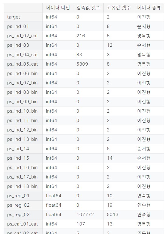
데이터 타입이 뭔지, 결측치가 몇개나 있는지, 교유값은 몇개인지, 데이터 종류가 이진형, 순서형, 명목형인지 한눈에 볼 수 있음
def write_percent(ax, total_size):
    #도형 객체를 순회하며 막대그래프 상단에 타깃값 비율 표시
    for patch in ax.patches:
        height = patch.get_height()
        width = patch.get_width()
        left_coord = patch.get_x()
        percent = height/total_size*100

        ax.text(left_coord + width/2.0,
               height + total_size*0.001,
               '{:1.1f}%'.format(percent),
               ha = 'center')

mpl.rc('font', size = 15)
plt.figure(figsize = (7, 6))

ax = sns.countplot(x = 'target', data = train)
write_percent(ax, len(train))
ax.set_title('Target Distribution')
타킷값이 0인 경우가 96.4로 3.6%인 1인 경우보다 압도적으로 많음
각 피쳐의 고유값별로 티킷값 1의 비율을 확인해서 피쳐와 타킷과의 관련성을 확인할 필요가 있음
신뢰구간이 너무 큰 경우 피쳐로 사용하지 않는 것이 좋을 수도 있음
import matplotlib.gridspec as gridspec

def plot_target_ratio_by_features(df, features, num_rows, num_cols, size = (12, 18)):
    mpl.rc('font', size = 9)
    plt.figure(figsize = size)
    grid = gridspec.GridSpec(num_rows, num_cols)
    plt.subplots_adjust(wspace = 0.3, hspace = 0.3)

    for idx, feature in enumerate(features):
        ax = plt.subplot(grid[idx])
        sns.barplot(x = feature, y = 'target', data = df, palette = 'Set2', ax = ax)
이진형 피처들의 고윳값별 타깃값 구하기
bin_features = summary[summary['데이터 종류'] == '이진형'].index
plot_target_ratio_by_features(train, bin_features, 6, 3)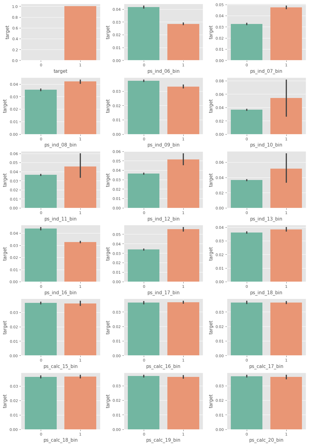
- ps_ind_10_bin ~ ps_ind_13_bin: 신뢰구간이 넓어서 통계적 유효성이 떨어짐
- ps_calc_15_bin ~ ps_calc_20_bin: 고윳값별 타깃값 비율 차이가 없어 타깃값 예측력 없음
명목형 피처들의 고윳값별 타깃값 구하기
nom_features = summary[summary['데이터 종류'] == '명목형'].index

plot_target_ratio_by_features(train, nom_features, 7, 2)
ps_car_10_cat: 세 고유값 간 비율이 비슷하기도 하고 고윳값 2의 신뢰구간이 유독 넓다.
순서형 피처들의 고윳값별 타깃값 구하기
ord_features = summary[summary['데이터 종류'] == '순서형'].index

plot_target_ratio_by_features(train, ord_features, 8, 2, (12, 20))
ps_ind_14: 고윳값 4의 타깃값 비율 신뢰구간이 넓어서 유효성 떨어짐
ps_calc_04 ~ ps_calc_14: 고윳값별 타깃값 비율 차이가 별로 없고, 차이나는 것은 신뢰구간이 너무 넓음
연속형 피처들의 고윳값별 타깃값 구하기
cont_features = summary[summary['데이터 종류'] == '연속형'].index

plt.figure(figsize = (12, 16))
grid = gridspec.GridSpec(5,2)
plt.subplots_adjust(wspace = 0.2, hspace = 0.4)

for idx, cont_feature in enumerate(cont_features):
    train[cont_feature] = pd.cut(train[cont_feature], 5) # 연속형 데이터들 5개의 구간으로

    ax = plt.subplot(grid[idx])
    sns.barplot(x = cont_feature, y = 'target', data = train, palette = 'Set2', ax=ax)
    ax.tick_params(axis = 'x', labelrotation = 10)
ps_calc_01 ~ ps_calc_03: 타깃값 비율 차이가 별로 없어서 제거하는 것으 좋을것 같음
연속형 피쳐 가 상관관계
plt.figure(figsize = (10, 8))
cont_corr = train_copy[cont_features].corr()
sns.heatmap(cont_corr, annot = True, cmap = 'OrRd');
데이터 합치기
all_data = pd.concat([train, test], ignore_index=True)
all_data = all_data.drop('target', axis=1) # 타깃값 제거

all_features = all_data.columns # 전체 피처
명목형 피쳐 원핫인코딩
from sklearn.preprocessing import OneHotEncoder

cat_features = [feature for feature in all_features if 'cat' in feature] # 명목형 피처

# 원-핫 인코딩 적용
onehot_encoder = OneHotEncoder()
encoded_cat_matrix = onehot_encoder.fit_transform(all_data[cat_features])
plus_features = ['ps_ind_02_cat', 'ps_ind_04_cat', 'ps_ind_05_cat',
'ps_car_01_cat', 'ps_car_01_cat', 'ps_car_07_cat', 'ps_car_09_cat']all_data_plus = all_data[plus_features]
all_data['num_missing'] = (all_data_plus == -1).sum(axis = 1)all_data.info()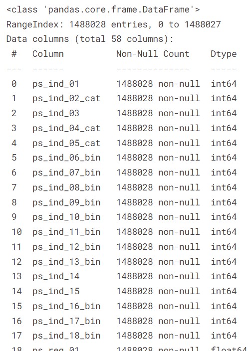
남길 피쳐 정리
remaining_features = [feature for feature in all_features
                      if ('cat' not in feature and 'calc' not in feature)]
remaining_features.append('num_missing')
mixed_ind 피쳐 만들기
ind_features = [feature for feature in all_features if 'ind' in feature]

is_first_feature = True
for ind_feature in ind_features:
    if is_first_feature:
        all_data['mix_ind'] = all_data[ind_feature].astype(str) + '_'
        is_first_feature = False
    else:
        all_data['mix_ind'] += all_data[ind_feature].astype(str) + '_'
all_data['mix_ind']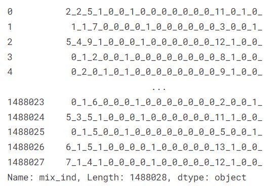
cat_count_features = []
for feature in cat_features+['mix_ind']:
    val_counts_dict = all_data[feature].value_counts().to_dict()
    all_data[f'{feature}_count'] = all_data[feature].apply(lambda x: val_counts_dict[x])
    cat_count_features.append(f'{feature}_count')
num_train = len(train)

train1 = all_data[:num_train]
X_test = all_data[num_train:]

train1['target'] = train['target'].values

train1.info()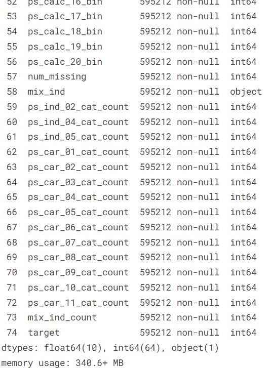
삭제할 피쳐 drop하기
from scipy import sparse

drop_features = ['ps_car_10_cat_count', 'ps_ind_10_bin', 'ps_ind_11_bin', 'ps_ind_13_bin', 'ps_ind_14']
all_data_remaining = all_data[remaining_features+cat_count_features].drop(drop_features, axis = 1)

all_data_sprs = sparse.hstack([sparse.csr_matrix(all_data_remaining),
                               encoded_cat_matrix],
                              format = 'csr')
트레인/테스트 데이터 나누기
num_train = len(train)

X = all_data_sprs[:num_train]
X_test = all_data_sprs[num_train:]

y = train['target'].values
- "결측값 개수"라는 파생피쳐 추가하기
- 해당 피쳐 내에서 해당 데이터가 속한 고윳값이 몇 개의 데이터를 가지고 있는지에 대한 파생피쳐 추가
- 신뢰구간과 고윳값별 타깃 비율의 차이 등을 검토해서 삭제할 피쳐 찾아
지니계수
import numpy as np

def eval_gini(y_true, y_pred):
    assert y_true.shape == y_pred.shape

    n_samples = y_true.shape[0]
    L_mid = np.linspace(1/n_samples, 1, n_samples)

    # 예측값에 대한 지니계수
    pred_order = y_true[y_pred.argsort()]
    L_pred = np.cumsum(pred_order) / np.sum(pred_order)
    G_pred = np.sum(L_mid - L_pred)

    # 예측이 완벽할 때 지니계수
    true_order = y_true[y_true.argsort()]
    L_true = np.cumsum(true_order) / np.sum(true_order)
    G_true = np.sum(L_mid - L_true)

    return G_pred / G_true
def gini(preds, dtrain):
labels = dtrain.get_label()
return 'gini', eval_gini(labels, preds)
xgboost 모델
import xgboost as xgb
from sklearn.model_selection import train_test_split

X_train, X_valid, y_train, y_valid = train_test_split(X, y, test_size = 0.2, random_state = 0)

bayes_dtrain = xgb.DMatrix(X_train, y_train)
bayes_dvalid = xgb.DMatrix(X_valid, y_valid)
하이퍼파라미터 후보들 (베이지안 사용예정)
param_bounds = {'max_depth': (4, 8),
                'subsample': (0.6, 0.9),
                'colsample_bytree': (0.7, 1.0),
                'min_child_weight': (5, 7),
                'gamma': (8, 11),
                'reg_alpha': (7, 9),
                'reg_lambda': (1.1, 1.5),
                'scale_pos_weight': (1.4, 1.6)}

fixed_params = {'objective': 'binary:logistic',
                'learning_rate': 0.02,
                'random_state': 1991}
def eval_function(max_depth, subsample, colsample_bytree, min_child_weight, reg_alpha, gamma, reg_lambda, scale_pos_weight):
params = {'max_depth': int(round(max_depth)),
'subsample': subsample,
'colsample_bytree': colsample_bytree,
'min_child_weight': min_child_weight,
'gamma': gamma,
'reg_alpha': reg_alpha,
'reg_lambda': reg_lambda,
'scale_pos_weight': scale_pos_weight}
params.update(fixed_params)
print('하이퍼파라미터:', params)
xgb_model = xgb.train(params = params,
dtrain = bayes_dtrain,
num_boost_round = 2000,
evals = [(bayes_dvalid, 'bayes_dvalid')],
maximize = True,
feval = gini,
early_stopping_rounds = 200,
verbose_eval = False)
best_iter = xgb_model.best_iteration
preds = xgb_model.predict(bayes_dvalid,
iteration_range = (0, best_iter)) # LIGHTGBM은 성능이 가장 좋을 때의 부스팅 반복 횟수 때의 모델을 예측때 알아서 사용하지만, XGBoost는 성능이 가장 좋을 때를 예측때 사용하라고 명시해줘야 함.
gini_score = eval_gini(y_valid, preds)
print(f'지니계수 {gini_score}\n')
return gini_scorefrom bayes_opt import BayesianOptimization
optimizer = BayesianOptimization(f = eval_function,
pbounds = param_bounds,
random_state = 0)
optimizer.maximize(init_points = 3, n_iter = 5)max_params = optimizer.max['params']
max_paramsmax_params['max_depth'] = int(round(max_params['max_depth']))
max_params.update(fixed_params)
max_paramsfrom sklearn.model_selection import StratifiedKFold
folds = StratifiedKFold(n_splits = 3, shuffle = True, random_state = 1991)
oof_val_preds = np.zeros(X.shape[0]) # 나중에 oof 방식으로 훈련된 모델로 검증 데이터 타깃값을 예측한 확률을 담을 1차원 배열
oof_test_preds = np.zeros(X_test.shape[0]) # 나중에 oof 방식으로 훈련된 모델로 테스트 데이터 타깃값을 예측한 확률을 담을 1차원 배열
for idx, (train_idx, valid_idx) in enumerate(folds.split(X, y)):
# 각 폴드를 구분하는 문구 출력
print('#'*40, f'폴드{idx+1} / 폴드 {folds.n_splits}', '#'*40)
# 훈련용 데이터, 검증용 데이터 설정
X_train, y_train = X[train_idx], y[train_idx]
X_valid, y_valid = X[valid_idx], y[valid_idx]
# XGBoost 전용 데이터셋 생성
dtrain = xgb.DMatrix(X_train, y_train)
dvalid = xgb.DMatrix(X_valid, y_valid)
dtest = xgb.DMatrix(X_test)
# XGBoost 모델 훈련
xgb_model = xgb.train(params = max_params, # 최적화로 찾은 파라미터 값을 적용
dtrain = dtrain,
num_boost_round = 2000,
evals = [(dvalid, 'valid')],
maximize = True,
feval = gini,
early_stopping_rounds = 200,
verbose_eval = 100)
# 성능의 가장 좋을 때의 부스팅 반복 횟수 저장해두기 -> 나중에 예측 때 사용
best_iter = xgb_model.best_iteration
# 테스트 데이터를 활용해 oof 예측
oof_test_preds += xgb_model.predict(dtest, iteration_range = (0, best_iter))/folds.n_splits
# 모델 성능 평가를 위한 검증 데이터 타깃값 예측
oof_val_preds[valid_idx] += xgb_model.predict(dvalid, iteration_range = (0, best_iter))
# 검증 데이터 예측 확률에 대한 정규화 지니계수
gini_score = eval_gini(y_valid, oof_val_preds[valid_idx])
print(f'폴드 {idx+1} 지니계수 : {gini_score}\n')print('OOF 검증 데이터 지니계수: ', eval_gini(y, oof_val_preds))submission['target'] = oof_test_preds
submission.to_csv('submission2.csv')